Data tables with Pandas#

Todo
Mystification
Data Manipulation#
We will learn to manipulate data, that is, a table with
attributes in columns and instances in rows in Python.
Pandas Library#
Pandas is a Python library that allows you to:
manipulate data tables, and
perform statistical analyses
as you could with a spreadsheet (Excel for example), but
programmatically, thus allowing automation.
Data tables (type DataFrame) are tables with two (or more)
dimensions, with labels (labels) on the rows and columns. The data is not necessarily
homogeneous: from one column to another, the type of data can
change (strings, floats, integers, etc.); in addition, some data
may be missing.
Series (type Series) are one-dimensional tables (vectors),
typically obtained by extracting a column from a DataFrame.
In this course, by table, we will mean a two-dimensional table of type
DataFrame, while by series we will mean a one-dimensional table of type
Series.
These concepts of DataFrame and Series are found in other libraries or
data analysis systems such as R.
In addition, Pandas allows you to process massive data distributed over very many
computers by relying on parallelism libraries such as
Data Series#
We must begin by importing the pandas library; it is traditional to define a shortcut
pd:
import pandas as pd
Let’s construct a series of temperatures:
temperatures = pd.Series([8.3, 10.5, 4.4, 2.9, 5.7, 11.1], name="Température")
temperatures
0     8.3
1    10.5
2     4.4
3     2.9
4     5.7
5    11.1
Name: Température, dtype: float64
Note that the series is considered as a column and the indices of its
rows are displayed. By default, these are the integers \(0,1,\ldots\), but other indices
are possible. As with C++ arrays or Python lists, we use the notation
‘t[i]’ to extract the row with index i:
temperatures[3]
np.float64(2.9)
The size of the series is obtained in the traditional way with Python using the
len function:
len(temperatures)
6
Let’s calculate the average temperature using the method mean:
temperatures.mean()
np.float64(7.1499999999999995)
Calculate the maximum temperature using the max method:
### BEGIN SOLUTION
temperatures.max()
### END SOLUTION
np.float64(11.1)
Calculate the minimum temperature:
### BEGIN SOLUTION
temperatures.min()
### END SOLUTION
np.float64(2.9)
What is the temperature data range?
### BEGIN SOLUTION
temperatures.max() - temperatures.min()
### END SOLUTION
np.float64(8.2)
Data tables (DataFrame)#
We will now construct a table containing the acidity data of water from
several wells. It will have two columns: one for the name of the wells and the other for the
pH value (acidity).
We can now build the table from the list of well names and
the list of well pH values:
df = pd.DataFrame({
    "Noms" : ['P1', 'P2', 'P3', 'P4', 'P5', 'P6', 'P7', 'P8', 'P9', 'P10'],
    "pH"   : [ 7.0,  6.5,  6.8,  7.1,  8.0,  7.0,  7.1,  6.8,  7.1,  7.1 ]
})
df
| Noms | pH | |
|---|---|---|
| 0 | P1 | 7.0 |
| 1 | P2 | 6.5 |
| 2 | P3 | 6.8 |
| 3 | P4 | 7.1 |
| 4 | P5 | 8.0 |
| 5 | P6 | 7.0 |
| 6 | P7 | 7.1 |
| 7 | P8 | 6.8 |
| 8 | P9 | 7.1 |
| 9 | P10 | 7.1 |
It is traditional to name
df(forDataFrame) the variable containing the table. But it is desirable to use a better name whenever natural!The first column of the table gives the index of the rows. By default, it is their number, starting at 0, in addition to the “Names” and “pH” columns.
This two-dimensional table is seen as a collection of columns. As a result,
df[label] extracts the column with the label label, in the form of a series:
df['Noms']
0     P1
1     P2
2     P3
3     P4
4     P5
5     P6
6     P7
7     P8
8     P9
9    P10
Name: Noms, dtype: object
You can then access each of the table’s values by specifying the label of
its column and then the index of its row. Here is the name in the second row (index 1):
df['Noms'][1]
'P2'
And the pH value in the fourth line (index 3):
df['pH'][3]
np.float64(7.1)
with a C++ array the access would be in the form t[ligne][colonne].
Metadata and Statistics#
We now use Pandas to extract some metadata and statistics from
our data.
First, the size of the table:
df.shape
(10, 2)
Column titles:
df.columns
Index(['Noms', 'pH'], dtype='object')
Number of lines:
len(df)
10
General information:
df.info()
<class 'pandas.core.frame.DataFrame'>
RangeIndex: 10 entries, 0 to 9
Data columns (total 2 columns):
 #   Column  Non-Null Count  Dtype
---  ------  --------------  -----
 0   Noms    10 non-null     object
 1   pH      10 non-null     float64
dtypes: float64(1), object(1)
memory usage: 292.0+ bytes
The average of each column for which it makes sense, that is to say only the
columns containing numerical values (here only the pH):
df.mean(numeric_only = True)
pH    7.05
dtype: float64
Standard deviations:
df.std(numeric_only = True)
pH    0.38658
dtype: float64
The median:
df.median(numeric_only = True)
pH    7.05
dtype: float64
The 25% quantile:
df.quantile(.25, numeric_only=True)
pH    6.85
Name: 0.25, dtype: float64
The minimum and maximum values:
df.min()
Noms     P1
pH      6.5
dtype: object
df.max()
Noms     P9
pH      8.0
dtype: object
A summary of the key statistics:
df.describe()
| pH | |
|---|---|
| count | 10.00000 |
| mean | 7.05000 |
| std | 0.38658 |
| min | 6.50000 |
| 25% | 6.85000 |
| 50% | 7.05000 |
| 75% | 7.10000 |
| max | 8.00000 |
The maximum pH index:
df['pH'].idxmax()
4
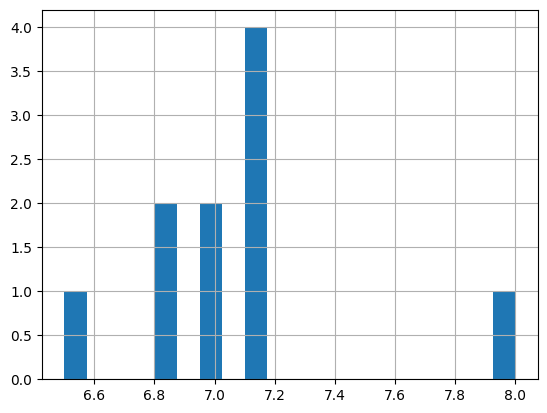
A histogram of the pH. Note: Here, we have the option bins = 20, which means that we
divide the range of pH (the x*-axis*) into 20 groups of the same size. Change the value of
bins to 2 and see the difference:
df['pH'].hist(bins=20);
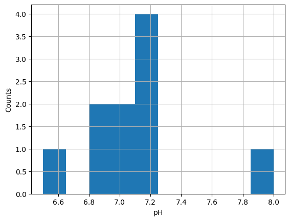
With pyplot, it is possible to refine the result by adding labels to the axes,
etc:
import matplotlib.pyplot as plt

df['pH'].plot(kind='hist')
plt.grid()
plt.ylabel('Counts')
plt.xlabel('pH');
Database operations#
Pandas allows you to perform database operations (for those who did the
Free Data project, remember “select”, “group by”, “join”, etc.). We
only show here the selection of rows; you will play with “group by” later.
Let’s transform the table so that one of the columns serves as indices; here we will
use the names:
df1 = df.set_index('Noms')
df1
| pH | |
|---|---|
| Noms | |
| P1 | 7.0 |
| P2 | 6.5 |
| P3 | 6.8 |
| P4 | 7.1 |
| P5 | 8.0 |
| P6 | 7.0 |
| P7 | 7.1 |
| P8 | 6.8 |
| P9 | 7.1 |
| P10 | 7.1 |
It is now possible to access a pH value by directly using the name
as a row index:
df1['pH']['P1']
np.float64(7.0)
Let’s now select all the pH \(7.1\) lines:
df1[df1['pH'] == 7.1]
| pH | |
|---|---|
| Noms | |
| P4 | 7.1 |
| P7 | 7.1 |
| P9 | 7.1 |
| P10 | 7.1 |
How does it work?
Let us denote pH the column with the same label:
pH = df1['pH']
pH
Noms
P1     7.0
P2     6.5
P3     6.8
P4     7.1
P5     8.0
P6     7.0
P7     7.1
P8     6.8
P9     7.1
P10    7.1
Name: pH, dtype: float64
As with NumPy, all operations are vectorized on all elements of the
array or series. Thus, if we write pH + 1 (which makes no
mathematical sense, the objects being of very different types: pH is a series while 1
is a number), this adds 1 to all the values of the series:
pH + 1
Noms
P1     8.0
P2     7.5
P3     7.8
P4     8.1
P5     9.0
P6     8.0
P7     8.1
P8     7.8
P9     8.1
P10    8.1
Name: pH, dtype: float64
Similarly, if we write pH == 7.1, this returns a series of booleans,
each indicating whether the corresponding value is equal to \(7.1\) or not:
pH == 7.1
Noms
P1     False
P2     False
P3     False
P4      True
P5     False
P6     False
P7      True
P8     False
P9      True
P10     True
Name: pH, dtype: bool
Finally, if you index an array by a series of booleans, it extracts the rows for which
the series contains True:
df1[pH == 7.1]
| pH | |
|---|---|
| Noms | |
| P4 | 7.1 |
| P7 | 7.1 |
| P9 | 7.1 |
| P10 | 7.1 |
Exercise: grades#
The Info 111 grades (anonymous!) from last year are in the CSV file notes_info_111.csv. Consult the content of this file:
You will notice that the values are separated by commas ‘,’ (CSV: Comma Separated
Value).
Here’s how to load this file as a Pandas table:
df = pd.read_csv("data/notes_info_111.csv", sep=",")
Display simple statistics in the:
### BEGIN SOLUTION
df.describe()
### END SOLUTION
| Total de Examen mi-semestre (EE) (Brut) | projet (CCTP) (Brut) | Note enseignant (Brut) | Outil externe Contrôle 1 PLaTon, jeudi 21 et vendredi 22 octobre (Brut) | Outil externe Contrôle 2 PLaTon, jeudi 9 - vendredi 10 décembre (Brut) | Total de Contrôles PLaTon (Brut) | Total de Note de TD (CCE) (Brut) | Total de Examen final (EEF) (Brut) | Total du cours (Brut) | |
|---|---|---|---|---|---|---|---|---|---|
| count | 276.000000 | 266.000000 | 272.000000 | 267.000000 | 267.000000 | 285.000000 | 286.000000 | 273.000000 | 286.000000 |
| mean | 13.715942 | 15.308271 | 15.978309 | 16.972846 | 17.319663 | 16.088035 | 15.631049 | 12.463004 | 13.420420 |
| std | 4.448350 | 4.625492 | 3.465690 | 4.306431 | 3.996111 | 5.528698 | 4.366991 | 5.763870 | 4.828153 |
| min | 0.600000 | 0.000000 | 5.000000 | 0.000000 | 0.000000 | 0.000000 | 0.000000 | 0.200000 | 0.000000 |
| 25% | 10.400000 | 13.000000 | 14.000000 | 16.150000 | 16.560000 | 15.260000 | 14.085000 | 7.800000 | 9.997500 |
| 50% | 14.000000 | 17.000000 | 16.550000 | 18.850000 | 19.060000 | 18.490000 | 16.915000 | 13.200000 | 14.395000 |
| 75% | 17.800000 | 19.000000 | 18.000000 | 19.620000 | 19.690000 | 19.530000 | 18.497500 | 18.000000 | 17.537500 |
| max | 20.000000 | 20.000000 | 20.000000 | 20.000000 | 20.000000 | 20.000000 | 20.000000 | 20.000000 | 20.000000 |
With DataGrid, you can interactively explore the table; try some of the following:
filtering ( icon);
sorting (click on the column header to sort by).
todo
verify datagrid for next year
from ipydatagrid import DataGrid
DataGrid(df)
Exercise: First names#
This exercise involves analyzing a database concerning first names
given in Paris between 2004 and 2018 (memories of S1?). This data is freely
accessible also on the
opendata site of the city of
Paris. The following shell command will download them into the
liste_des_prenoms.csv file if it is not already present.
if [ ! -f liste_des_prenoms.csv ]; then
    curl --http1.1 "https://opendata.paris.fr/explore/dataset/liste_des_prenoms/download/?format=csv&timezone=Europe/Berlin&lang=fr&use_labels_for_header=true&csv_separator=%3B" -o data/liste_des_prenoms.csv
fi
Open the file to view its contents.
Using the example above as inspiration, import the file
data/liste_des_prenoms.csvinto a tableprenoms. Note: the file uses semicolons;as separators and not commas,.
### BEGIN SOLUTION
prenoms = pd.read_csv('data/liste_des_prenoms.csv', sep=';')
### END SOLUTION
If the test below fails, please verify that you have correctly named your array
prenoms (without accent, with an s):
assert isinstance(prenoms, pd.DataFrame)
assert list(prenoms.columns) == ['Nombre prénoms déclarés', 'Sexe', 'Annee', 'Prenoms','Nombre total cumule par annee']
Display the first ten lines of the file. Hint: consult the documentation of the
headmethod usingprenoms.head?
### BEGIN SOLUTION
prenoms.head(10)
### END SOLUTION
| Nombre prénoms déclarés | Sexe | Annee | Prenoms | Nombre total cumule par annee | |
|---|---|---|---|---|---|
| 0 | 179 | M | 2024 | Isaac | 179 |
| 1 | 125 | M | 2024 | Paul | 125 |
| 2 | 83 | F | 2024 | Lina | 83 |
| 3 | 78 | F | 2024 | Victoria | 78 |
| 4 | 77 | M | 2024 | Aylan | 77 |
| 5 | 68 | M | 2024 | Zayn | 68 |
| 6 | 61 | F | 2024 | Inaya | 61 |
| 7 | 60 | F | 2024 | Mariam | 60 |
| 8 | 55 | F | 2024 | Inès | 55 |
| 9 | 48 | M | 2024 | Orso | 48 |
Display the lines corresponding to your first name (or another first name such as Mohammed, Maxime or even Brune if your first name is not in the list):
### BEGIN SOLUTION
prenoms[prenoms.Prenoms == "Brune"]
### END SOLUTION
| Nombre prénoms déclarés | Sexe | Annee | Prenoms | Nombre total cumule par annee | |
|---|---|---|---|---|---|
| 655 | 7 | F | 2006 | Brune | 7 |
| 712 | 11 | F | 2007 | Brune | 11 |
| 1037 | 20 | F | 2010 | Brune | 20 |
| 2785 | 25 | F | 2015 | Brune | 25 |
| 3601 | 53 | F | 2018 | Brune | 53 |
| 3771 | 26 | F | 2016 | Brune | 26 |
| 3869 | 50 | F | 2019 | Brune | 50 |
| 7527 | 42 | F | 2021 | Brune | 42 |
| 8048 | 44 | F | 2020 | Brune | 44 |
| 14110 | 27 | F | 2012 | Brune | 27 |
| 14246 | 23 | F | 2014 | Brune | 23 |
| 14918 | 20 | F | 2011 | Brune | 20 |
| 15955 | 6 | F | 2004 | Brune | 6 |
| 17181 | 26 | F | 2017 | Brune | 26 |
| 20948 | 18 | F | 2013 | Brune | 18 |
| 21774 | 16 | F | 2008 | Brune | 16 |
| 22038 | 10 | F | 2005 | Brune | 10 |
| 22830 | 18 | F | 2009 | Brune | 18 |
| 23317 | 55 | F | 2022 | Brune | 55 |
| 25488 | 40 | F | 2023 | Brune | 40 |
| 26008 | 42 | F | 2024 | Brune | 42 |
Do the same interactively with
DataGrid:
DataGrid(prenoms)
Extract the female first names (with repetitions) into a variable
prenoms_femmes, in the form of a series. Hint: see in the examples above how to select rows and how to extract a column.
### BEGIN SOLUTION
prenoms_femmes = prenoms['Prenoms'][prenoms['Sexe'] == 'F']
prenoms_femmes
### END SOLUTION
2            Lina
3        Victoria
6           Inaya
7          Mariam
8            Inès
           ...
26669      Saskia
26672       Edmée
26673       Enola
26674        Gala
26675       Perla
Name: Prenoms, Length: 13583, dtype: object
How many are there?
### BEGIN SOLUTION
len(prenoms_femmes)
### END SOLUTION
13583
# Vérifie que prenoms_femmes est bien une série
assert isinstance(prenoms_femmes, pd.Series)
# Vérifie le premier prénom alphabetiquement
assert prenoms_femmes.min() == 'Aaliyah'
# Vérifie le nombre de prénoms après suppression des répétitions
assert len(set(prenoms_femmes)) == 1491
Do the same for men’s first names:
### BEGIN SOLUTION
prenoms_hommes = prenoms['Prenoms'][prenoms['Sexe']=='M']
prenoms_hommes
### END SOLUTION
0         Isaac
1          Paul
4         Aylan
5          Zayn
9          Orso
          ...
26666     Nahel
26670    Aharon
26671      Theo
26676     Marlo
26677     Viggo
Name: Prenoms, Length: 13095, dtype: object
### BEGIN SOLUTION
len(prenoms_hommes)
### END SOLUTION
13095
A quick check:
assert len(prenoms_hommes) + len(prenoms_femmes) == len(prenoms)
Exercise: Transform the first names to uppercase in the table prenoms. Assign the
result
to the variable prenoms_maj
Objective: Know how to search in the pandas documentation:
https://pandas.pydata.org/docs/user_guide/.
### BEGIN SOLUTION
# Solution apres avoir cherche dans "working with text" in the user guide
prenoms_maj = prenoms['Prenoms'].str.upper()
### END SOLUTION
Exercise \(\clubsuit\)
What is the most declared first name, cumulatively across all years? Assign it to the
variable prenom
Hint: consult the first example at the end of the documentation of the
groupby method to calculate the cumulative numbers by first name (with sum). Then use
DataGrid to visualize the result and sort it, or use sort_values, or
idxmax
### BEGIN SOLUTION
df = prenoms.groupby('Prenoms').sum()
# Solution 1
DataGrid(df)
# Solution 2
df.sort_values("Nombre prénoms déclarés")
### END SOLUTION
| Nombre prénoms déclarés | Sexe | Annee | Nombre total cumule par annee | |
|---|---|---|---|---|
| Prenoms | ||||
| Norhane | 5 | F | 2013 | 5 |
| Celina | 5 | F | 2008 | 5 |
| Chad | 5 | M | 2004 | 5 |
| Chaden | 5 | F | 2015 | 5 |
| Saly | 5 | F | 2018 | 5 |
| ... | ... | ... | ... | ... |
| Arthur | 5235 | MMMMMMMMMMMMMMMMMMMMM | 42294 | 5235 |
| Louise | 5373 | FFFFFFFFFFFFFFFFFFFFF | 42294 | 5373 |
| Adam | 5857 | MMMMMMMMMMMMMMMMMMMMM | 42294 | 5857 |
| Raphaël | 5887 | MMMMMMMMMMMMMMMMMMMMM | 42294 | 5887 |
| Gabriel | 7087 | MMMMMMMMMMMMMMMMMMMMM | 42294 | 7087 |
2823 rows × 4 columns
### BEGIN SOLUTION
# Solution 3
prenom = df['Nombre prénoms déclarés'].idxmax()
### END SOLUTION
This test verifies that you have found the correct answer; without giving it to you; the magic of hash functions :-)
import hashlib
assert hashlib.md5(prenom.encode("utf-8")).hexdigest() == 'b70e2a0d855b4dc7b1ea34a8a9d10305'
Conclusion#
Todo
qu’est-ce qui a été vu dans cette feuille?